

Geometry from order: causal sets
An overview of the causal set approach to a theory of quantum gravity
An article by Rafael Sorkin
Among the various ideas put forward in the search for a theory of quantum gravity, the causal set hypothesis is distinguished by its logical simplicity and by the fact that it incorporates the assumption of an underlying spacetime discreteness organically and from the very beginning.
In the way that it has developed, the causal set hypothesis has given rise to a mathematical framework (the “dynamics of sequential growth”) in which time is an active process of “becoming” that can be identified with the continual birth of new elements of the causal set.
The conceptual simplicity of the theory has meant that it has been possible to draw from it interesting phenomenological consequences, even though the theory remains in an incomplete stage of development. Perhaps the most interesting prediction so far was that of fluctuations in the value of the so-called cosmological constant that are consistent with subsequent observations.
From Zeno to Causets
The basic ideas behind the concept of a causal set (which has come to be known as a “causet”) have a long history. The idea that space might be discrete goes back at least to Zeno, and in more recent times Bernhard Riemann wrote in 1854, in a lecture that laid the foundations of the geometry of curved spaces,
“The question of the validity of the presuppositions of geometry in the infinitely small hangs together with the question of the inner ground of the metric relationships of space. In connection with the latter question… the above remark applies, that for a discrete manifold, the principle of its metric relationships is already contained in the concept of the manifold itself, whereas for a continuous manifold, it must come from somewhere else. Therefore, either the reality which underlies physical space must form a discrete manifold or else the basis of its metric relationships should be sought for outside it[…].”
Here Riemann is asking what it is about the structure of space that makes it possible to talk about measurable things like distance, area, volume and angles (the “metric relationships”), and he is contrasting the case in which the deep structure of space is continuous with the case in which it is discrete. In a continuous space (like that of Euclidean geometry) there are between any two points always an infinity of others, and every volume can be divided into smaller and smaller volumes without limit. In a discrete space, in contrast, any bounded region is composed of a finite number of elements or “building blocks”, and the process of subdivision must always come to an end at some stage. Riemann’s point, then, is that a discrete space has metric information built in from the start. It is easy to see the truth of this: For instance, simply counting the elements composing a region of space provides a natural measure of that region’s volume. For a continuous space, in contrast, this possibility to count elements is lacking (you’d just get infinity for the answer) and the origin of the metric relationships has to be explained in some other manner.
A century later, Einstein, who had taken over Riemann’s concept of a continuous curved space for the theory of general relativity (but now as spacetime rather than just space) also doubted whether, deep down, continuity could persist:
“In any case, it seems to me that the alternative continuum-discontinuum is a genuine alternative; i.e. there is no compromise here. In [a discontinuum] theory there cannot be space and time, only numbers[…]. It will be especially difficult to elicit something like a spatio-temporal quasi-order from such a schema. I can not picture to myself how the axiomatic framework of such a physics could look[…]. But I hold it as altogether possible that developments will lead there[…].” [Reference]
(Einstein here calls “discontinuum” what Riemann calls “discrete manifold”.)
We find in these quotations all the ingredients of the causet hypothesis: that spacetime might not be an ultimate reality; that what Riemann calls a discrete manifold might be its inner basis; that in this case the metric relationships are inherent in the discrete manifold itself; and that it is important to be able to deduce the temporal ordering of spacetime events from the deeper structure. When the deeper structure is a causet this last requirement is, despite Einstein’s misgivings, not especially difficult, because a causet incorporates an order relation by its very definition. Indeed it is this order relation.
A causet, to be more precise, is a discrete set of elements – the basic spacetime building blocks or “elementary events“. But whereas in the continuum, spacetime is described, mathematically speaking, by an elaborate web of relationships among the point-events carrying information about contiguity, about smoothness, and about distances and times, for the elements of a causet the only relational information we have is what mathematicians call a “partial (or quasi-) order” – for some pairs x, y of elements (not for all!) we have the information that x comes before y, or, in other cases, that x comes after y. Physically, you should think of this ordering as a microscopic counterpart of the macroscopic relation of before and after in time: For some events, we know that they take place after certain other events. (The word “causal” comes in because we say that an event is later than another event if the latter could exert a causal influence on the former.)
Geometry from order and number
What is remarkable is that this structure alone suffices to reproduce (to a high degree of approximation) everything that we mean by the geometry of spacetime.
I cannot explain this claim fully here, but its basis can be indicated by the slogan “Order + Number = Geometry”. To get an idea of where this remarkable equation comes from, you must realize first that, according to general relativity, the local geometry of spacetime (or equivalently the gravitational field), can be defined by 10 numbers to be specified at each spacetime point. To capture the geometry is therefore to capture these ten numbers.
Now, nine of these numbers can be reconstructed from a knowledge of how light propagates through spacetime, for the simple reason that the geometry of spacetime governs the way that light propagates.
Let us pause for a minute to consider this further. Knowing how light propagates means knowing what is called the light-cone at every spacetime point. All the possible light signals that can be sent from (or received) at a certain spacetime point (a certain point in space at a certain time) together trace out a double cone. Since light has the maximum possible speed, this cone divides the neighbourhood of that particular spacetime point into separate regions, as indicated in the following illustration:

In the illustration, the vertical axis stands for time (in a particular reference frame), while the horizontal axis represents one of the spatial directions (with respect to the same reference frame). Light signals (in other words, their world lines) are represented by straight lines. No event in region III can be the cause of anything that happens at our spacetime point, since any influence would have had to travel faster than light. On the other hand, any event in region II can, in principle, influence our spacetime point, while anything that happens at our spacetime point can influence anything that happens in region I. But such a causal structure is exactly what is encoded in the partial ordering of the causet elements: The statement that “event A comes before B” is equivalent to saying that “B is in the light-cone of event A, in region I”. “Event A comes after B” means “B is in the light-cone of event A, in region II”. That no order is defined between A and B means that in the light-cone of event A, event B is in region III (and vice versa).
Thus, if we know which events temporally precede which others (in the sense that they can influence them), we know the light cones, and vice versa. Thus – to return to the main question – if we know the causal ordering among events, then we know the light-cones and we therefore know nine of the ten numbers necessary to describe the geometry of spacetime.
The missing information, namely information on spacetime volume, comes by counting – the spacetime volume of a region is simply the number of causet elements comprising that region, in brief: volume = number. Thus, to oversimplify slightly, in the equation
Order + Number = Geometry
the order carries 9/10 of the information and the number 1/10. Together they add up to 10/10. Notice that all this makes sense only because a causet is discrete. Were it continuous, each portion of spacetime would consist of an infinite number of elements, and counting them would have no meaning.
To get a feel for the numbers involved in this kind of counting, observe that a region of spacetime of spatial volume one cubic centimetre and a temporal extent of one second is composed of around 10139 elements, an unimaginably big number, but still finite. This would explain why we haven’t yet noticed the granularity of spacetime, even in laboratories.
From kinematics to dynamics: Sequential growth
The kind of order relation that defines a causet can be viewed as a pattern of ancestral relationships so that, when an element x temporally precedes an element y, we say that x is an ancestor of y. It is thus natural to depict a causet as a generalized family tree (known in mathematics as a Hasse diagram). Here is a very simple causet of only ten elements, drawn this way. In this causet, the ancestors of element a, for example, are elements b, c, and d: a happens after each of the events b, c and d. (Time flows upward in these diagrams, just as it does in the analogous, but more familiar spacetime diagrams, but opposite to how family trees are often drawn.)

But all this so far is just what physicists would call “kinematics without dynamics”: It describes what a causet is (and how it relates to a spacetime), but not how it develops. In the dynamical scheme that has emerged from recent work in causet theory, this development appears as a “growth process” in which elements are born one at a time. Here, for example is a succession of births that could have given rise to the causet depicted above (call it C):

The growth starts from nothing, and each element that comes into being is born with a definite set of immediate ancestors or “parents” (as indicated by the descending lines). An element cannot be born before any of its ancestors (rule of “internal temporality”). Other than that, the order of birth is arbitrary.
It is very important, however, that what is shown in this animation is not the only way that C might have grown. The following animation shows two different possible growth sequences in parallel:

If time has no physical meaning except as represented in the causal relations themselves, then these two movies are not physically distinct; they are just different ways of representing the same process.
This equivalence is, in the discrete setting of causets, an exact correspondent of what is called the principle of general covariance in ordinary, continuous spacetime – the statement that all the infinitely many possibilities of choosing numbers (coordinates) to label the point-events of spacetime are equivalent.
In the continuum, this principle (when suitably supplemented) leads more or less uniquely to the Einstein equations for spacetime. For causets, it leads (when suitably supplemented) to a family of dynamics called classical sequential growth (CSG) models. As the adjective “classical” indicates, these models do not yet incorporate the principles of quantum theory, and a major aim of current work on causal set theory is to take this last step and produce an appropriate quantum version of the CSG models. If this can be done, we will have a fully fledged theory of quantum gravity.
Consequences and applications
Even at the present stage of development of the theory, though, certain phenomenological conclusions can already be drawn from it. One of the earliest of these was the prediction already mentioned, concerning the cosmological constant – a phrase that denotes a possible modification of the law of gravity that Einstein had considered and later rejected. The following figure illustrates this prediction:
![[Figure from M. Ahmed et al., Physical Review D69, 103523 (2004); astro-ph/0209274 / Redesign: Daniela Leitner for Einstein Online]](https://www.einstein-online.info/wp-content/uploads/Relativity_and_the_quantum_Expansion_©_M_Ahmed_et_al_Physical_Review_D69_103523_2004_astro-ph_0209274_Redesign_Daniela_Leitner_Einstein-Online.jpg "[Figure from M. Ahmed et al., Physical Review D69, 103523 (2004); astro-ph/0209274 / Redesign: Daniela Leitner for Einstein Online]")
[Figure from M. Ahmed et al., Physical Review D69, 103523 (2004); astro-ph/0209274 /
Redesign: Daniela Leitner for Einstein Online]
Until recently cosmologists had almost universally omitted the cosmological constant from their models without even mentioning that they were doing so, but everything changed when supernova observations began to indicate that gravity (in the present cosmological epoch) ceases to be attractive at large distances. This behavior can be attributed to a cosmological constant of precisely the order of magnitude that had been anticipated from causet theory. This order of magnitude agrees with that of the energy density of matter and radiation today. But as seen in the figure above, the same approximate equality would have held throughout the history of the universe, thereby resolving what cosmologists have called the “why now?” puzzle.
Another prediction from causal sets is that particles should in principle swerve slightly in their motion, and do so in a random manner that has a very precise mathematical description, of the sort that applies to a molecule diffusing through a fluid.
The growth models we have so far also point to a possible explanation for the large size and great uniformity of the cosmos. According to this idea, what we call the big bang would only mark the beginning of the most recent in a long series of cycles of cosmic expansion and recontraction. In each cycle the cosmos would expand to a larger size, and the fact that it is now so big would merely reflect the large number of cycles preceding ours.
Our current understanding also points to the need for modifications of quantum field theory (the type of theory that describes subatomic particles and fields). They introduce a kind of limited action at a distance (nonlocality) which would reach over distances which are still very small, but nonetheless much bigger than the Planck length that is usually associated with quantum gravity effects (about 10-32 cm).
A model for the way that the horizon of a black hole might be composed of discrete building blocks (derived directly from the causet elements themselves) also emerges naturally from causet kinematics.
Finally, it’s worth returning briefly to a philosophical consequence of the CSG models that I alluded to earlier. One often hears that the principle of general covariance (or even just its special case in special relativity, Lorentz invariance) forces us to abandon “becoming” (in German, “Werden”) and view spacetime as static – with the whole past and future all laid out in one timeless tableau. To this claim, the CSG dynamics provides a counterexample. It refutes the claim because it offers us an active process of growth in which “things really happen”, but at the same time it honors general covariance. In doing so, it shows how the “Now” might be restored to physics without paying the price of a return to the absolute simultaneity of pre-relativistic days.
Further Information
For the basic concepts of relativity of interest for this spotlight topic, check out Elementary Einstein, in particular the chapter Relativity and the quantum .
Related Spotlights on relativity on Einstein-Online can be found in the section Relativity and the quantum.
Reference
Einstein, Letter to H.S. Joachim, August 14, 1954, Item 13-453, cited in J. Stachel, “Einstein and the Quantum: Fifty Years of Struggle”, in (R. G. Colodny, ed.). U. Pittsburgh Press 1986), pp. 380-381.
Colophon
is emeritus professor of physics at Syracuse University, New York State, and a senior researcher at the Perimeter Institute for Theoretical Physics in Waterloo, Canada. His research focuses on the causal set hypothesis as the basis of a theory of quantum gravity.
Citation
Cite this article as:
Rafael Sorkin, “Geometry from order: causal sets” in: Einstein Online Band 02 (2006), 02-1007
Weitere Artikel
 Relativity and the Quantum / Elementary Tour part 1: Relativity in the micro-world
 Searching for the quantum beginning of the universe
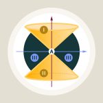 Special relativity / Elementary Tour part 5: Spacetime
 Kosmologie / Einsteiger-Tour Teil Fazit
- Special relativity / Elementary Tour: Conclusion
- Relativity and the Quantum / Elementary Tour: Conclusion