Cosmic Sound: Curvature and the cosmic background radiation

How the spatial geometry of the universe can be derived by observing the cosmic background radiation

An article by Matthias Bartelmann

For the first 400,000 years after the big bang, the universe was so exceedingly hot that no stable atoms could exist. Instead, the cosmos was filled with elementary particles and, during all but the first minute of that era, with a plasma consisting of electrons and atomic nuclei. Also, there were photons and particles of what is called dark matter, as well as a number of other species of elementary particles that will not be important for what we are about to explore in this text.

The only way that dark matter interacts with ordinary matter is via gravity. On the other hand, a mixture of photons and electrically charged particles – such as electrons and nuclei – is subject to intense electromagnetic interactions. Consequently, the universe was completely opaque until it had cooled down sufficiently for electrons and nuclei to combine into stable atoms.

Quite soon after the big bang, the distribution of dark matter in the universe started to develop inhomogeneities, with the dark matter density slightly above average in some regions and slightly below in others. These density fluctuations were the first seeds of the large-scale structure that we observe in the cosmos today, where matter is concentrated in galaxies and galaxy clusters. But the fluctuations also had important short-term consequences: They excited oscillations in the cosmic plasma.

Plasma oscillations

The oscillations came about in the following way: Regions of higher dark matter density cause increased gravitational attraction. In consequence, the plasma density increases in such regions as well: As plasma flows into the region, it gets compressed. Compressed plasma has a higher internal pressure, chiefly due to the photons but also transferred to the plasma itself via electromagnetic interaction. Once the pressure has increased sufficiently, it drives the plasma particles apart, leading to lower-than-average plasma density in that particular region. The plasma pressure drops as well, and thus, by its gravitational attraction, the dark matter can again pull more plasma into the region – thereby increasing the plasma density -, and the cycle can start anew. The resulting plasma oscillations are very similar to sound waves – sound waves, after all, are propagating, periodic density fluctuations in air. Therefore, physicists call these plasma oscillations “acoustic oscillations”.

Sound waves travel at the speed of sound c_s. For ordinary sound waves in air, this amounts to around 300 metres per second. In contrast, for the plasma sound waves in the early universe, the speed of sound amounts to roughly 60% of the speed of light. The speed of sound tells us how fast existing density perturbations travel through space. But it also tells us how long it takes to excite specific oscillations: It takes a region of spatial extension L a time L/c_s to settle into a coherent state of oscillation in which the plasma density increases and decreases in the same way throughout the whole region.

This leads to an upper limit for the spatial extent of any acoustic oscillation in the early universe. The reason is that there was only a limited time, the aforementioned 400,000 years, for these oscillations to be excited in the cosmic plasma. After that period of time, the plasma particles combined to form stable atoms. Since the strong electromagnetic coupling between photons and matter depended on the presence of free electric charges (photons are constantly being absorbed and re-emitted by charged particles), the formation of atoms meant that the strong coupling of photons and matter came to an end. There was an abrupt drop in pressure, and the oscillations ceased.

At the close of those 400,000 years, the largest possible coherent oscillations had a spatial extent of 230,000 lightyears (or 70,000 parsec). There was simply no time for more: With the speed of sound at 60% light speed and a time of roughly 400,000 years, the largest regions in which coherent oscillations could develop had a spatial extent of 0.6·400,000 = 240,000 lightyears; with the more precise value of 380,000 years for the cosmic time when atoms formed, the result is 230,000 lightyears. This upper limit is called the “sound horizon”.

What’s in it for cosmology?

The main reason these oscillations are of great interest to cosmology is that astronomers can measure the apparent size of the sound horizon in the sky. The photons that were set free in the transition from a cosmic plasma to stable atoms make up the cosmic microwave background radiation which is present everywhere in the cosmos. As we detect this radiation in the sky, we are practically looking at a snapshot of the early universe. The radiation is thermal – its spectrum depends only on a single parameter, the radiation temperature (further information about this type of radiation can be found in the spotlight text Heat that meets the eye).

When the first stable atoms formed, the sound waves in the cosmic plasma caused tiny fluctuations in the temperature of the cosmic microwave background: The temperatures of the radiation reaching us from different regions in the sky typically differ by some hundredth or tenth of a thousandth Kelvin (equivalently, degrees Celsius). With satellites like the European Planck, astronomers can map those temperature differences with high precision. Here is the result:

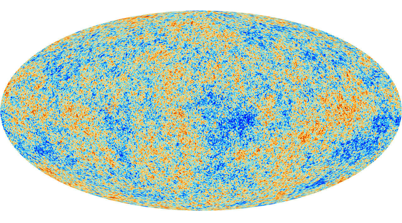
[Image: ESA, Planck collaboration]

In this image, the sky is projected onto a flat surface in the same way that the spherical earth can be projected to create a map. Blueish regions indicate radiation temperatures below, reddish regions temperatures above average.

The fluctuation pattern visible in the image results from a combination of all the different acoustic oscillations in the early universe – from those with the smallest to those with the largest spatial size. Through a careful analysis similar to the frequency analysis for ordinary sound waves, it is possible to extract from this map the contribution from each of the different oscillations. The oscillation with the largest spatial extent indicates the size of the sound horizon.

However, what can be measured in this way is not the absolute size of the sound horizon, but merely its angular size in the sky. We do know the absolute size already, namely the 230,000 lightyears mentioned above. This is a highly interesting combination, since by comparing the angular and the absolute sizes, cosmologists can determine the curvature of our cosmos – whether space is flat, or has a sphere-like or saddle-like shape (some information about these possibilities can be found in the spotlight text The shape of space).

In ordinary, Euclidean space (“flat space”), we are well acquainted with the relationship: The angular size (the “apparent size”) of a given object decreases linearly with the distance – at least for far-away objects. The following image shows the relationship between the spatial extent L of a measuring rod, its distance and its angular size α. Shown in red are light rays connecting us, the observer, with both ends of the measuring rod:

Matters are somewhat different in a space of positive curvature, the three-dimensional analogue of a spherical surface. In such a space, light does not travel along straight lines. Instead, light rays converge, as can be seen in this image:

In such a space, the same measuring rod at the same distance from us will have a larger apparent size, corresponding to a larger angle α.

In a space with negative curvature, it is the other way round: Light rays diverge, and as a result the same measuring rod, still at the same distance, will have a smaller apparent size, corresponding to smaller α:

Consequently, it is simple to read off the curvature of space from the cosmic microwave background: We know the absolute size of the largest sound waves in the early universe, and we can measure their apparent size in the sky. The distance of the microwave background can be calculated: We know the temperature at which it was formed, and we can measure its temperature today. The temperature difference is directly related to the amount by which the universe has expanded from then until now, and this, in turn, is directly related to the distance. Comparing the apparent and true sizes at the calculated distance, we obtain the curvature of space. In this way, astronomers have determined that, to high precision, space in our cosmos is flat.

Further Information