Waves, motion and frequency: the Doppler effect
How motion influences waves, or other kinds of ever-repeating signals, in classical physics and in special relativity.
An article by Markus Poessel
The frequency of a wave-like signal – such as sound or light – depends on the movement of the sender and of the receiver. This is known as the Doppler effect. Some of its manifestations, we know from everyday life, such as a fire engine’s siren abruptly changing pitch as the engine passes by; others are of interest in astronomy and astrophysics. The purpose of this spotlight text is to take a closer look at what the Doppler effect is all about.
Pulses sent out and received
We will start with a very simple set-up, which you can see in the following animation. On the right-hand side, drawn in red, there is a sender that emits pulses in regular succession. On the left-hand side there is a receiver, drawn in blue. The pulses themselves are drawn in red, and they all travel at the same speed from right to left. Everytime the sender emits a new pulse, a indicator light flashes once. Likewise, a flashing light indicates when a pulse has reached the receiver:

If you observe first the indicator at the detector, and then the indicator flashing at the receiver, you can verify that they both flash with the same rhythm, in other words: The time between the emission of two successive pulses is the same as the time between the reception of two such pulses.
Putting the same statement into other words: The frequency with which the pulses are emitted – the number of pulses emitted in a certain period of time, for example in one second – is the same as the frequency with which they are received.
Pulses from an approaching source
Next, let us look at a slightly different situation, where the source is moving towards the detector. We assume that the motion of the sender does not influence the speed at which the pulses travel, and that the pulses are sent with the same frequency as before. Still, as we can see in the following animation, the motion influences the pulse pattern:

The distance between successive pulses is now smaller than when both sender and receiver were at rest. Consequently, the pulses arrive at the receiver in quicker succession. If we compare the rates at which the indicator lights at the receiver and at the sender are flashing, we find that the indicator light at the receiver is flashing faster.
More concretely, in this situation the sender is moving to the left at a third the speed of the pulses. During the time it takes two pulses to be sent out from the sender, three pulses have arrived at the receiver. Put differently: The frequency at which the pulses are received is 3/2=1.5 times the frequency at which they are emitted. The frequency has shifted – which is why the Doppler effect is often referred to as the Doppler shift.
How does this come about? Let us go back to the case of the non-moving sender. Here is a snapshot of the sender emitting one pulse:

After some time interval T has passed, the sender will emit a second pulse, as pictured here. In the meantime, the first pulse will have moved a distance d to the left:

The distance d determines the time it takes two successive pulses to arrive at the receiver. All the pulses are travelling at the same speed, and the time between two arrivals is simply the time it takes the second pulse to cover the distance d. The larger d, the longer the time that will pass between the arrivals of two successive pulses. The larger the distance between two successive pulses, the lower the frequency of pulse arrival – if the pulses are separated by a large distance, only a comparatively small number of them will reach the receiver in a given time.
So far, so good. But what if the sender is moving? Again, here is a snapshot of the moving source emitting one pulse:
After the same time interval T has passed, the sender will emit a second pulse. In the meantime, the first pulse has, again, moved a distance d to the left. But in this case it is not the only thing that has moved. The sender itself has moved left by a certain distance D, as sketched here:

Due to the sender’s motion, the distance between two successive pulses in this case is not d, but d-D. But when the distance between successive pulses is smaller, the time interval that passes between their arrival at the detector is also smaller or, put differently, the frequency with which the pulses arrive at the detector is higher!
This is our first example for the Doppler effect: When the sender is moving towards the receiver, the frequency with which the pulses reach the receiver is higher than the frequency with which they are emitted by the sender.
Source moving away from receiver
What if the source is not moving towards, but away from the receiver? This situation is shown in the following animation:

This time, the receiver’s indicator light blinks a bit slower than the sender’s – the frequency with which the pulses are received is a bit lower than the one with which they are sent out. More precisely, the source is moving to the right at one third the speed with which the pulses travel to the left. During the same time that four pulses are sent out, three pulses are received.
This is readily understood in the same way as before. Here, once more, is a snapshot of the source emitting one specific pulse:
After the time T has passed, a second pulse is emitted. During that time, the first pulse has, once more, travelled the distance d. But in addition, the source has moved a distance D to the right:

Thus, the distance between two successive pulses is now larger than for a non-moving source – it is d+D instead of just d. But a larger distance means that the pulses arrive at the receiver less frequently. This is our second example for the Doppler effect: When the sender is moving away from the receiver, the frequency with which the pulses reach the receiver is lower than the frequency with which they are emitted by the sender.
From pulses to waves
Now imagine that, instead of separate pulses, our sender is emitting a simple wave – a travelling pattern, maxima and minima (crests and troughs) of some physical quantity following each other with perfect regularity and propagating at some constant speed through space:

For instance, our sender could be emitting a sound wave, in which the wave’s crests and troughs would correspond to regions of maximal or minimal air pressure, respectively. Such a sound wave would travel at a constant speed, the speed of sound, through the air. Alternatively, our sender could be emitting an electromagnetic wave, where the crests and troughs correspond to locations of a maximum or minimum value of a more abstract physical quantity, either the electric or the magnetic field. One example for such an electromagnetic field would be ordinary light.
One key insight is that all the arguments we have made about the emission of pulses apply to the emission of subsequent wave crests (or wave troughs), as well. For instance, if the source is moving towards the receiver, it will emit each wave crest somewhat closer to its immediate predecessor than if the source were at rest. This brings us to the more common version of the Doppler effect, the one that talks about waves: If the source of a wave is moving towards a receiver, the frequency at which the waves are received is higher than the frequency at which they are sent out. Conversely, if the source is moving away, then the frequency at which the waves are received is lower.
For sound waves, many readers will have first-hand experience with this phenomenon. For these waves, higher frequency corresponds to a higher pitch, lower frequency to a lower pitch. Assume that you are standing near a road where a fire truck or police car is passing. As the car comes towards you, then passes you, and finally moves away from you, you can distinctly hear how the pitch of its siren starts out higher and then quite abruptly drops lower.
Play [MP3, 258 kB], Download [ZIP, 184kB]
For simple light waves, frequency is related to color. The lowest possible frequency of visible light corresponds to reddish light. As we go to higher frequencies, we traverse the visible spectrum from red to yellow, green, blue and violet, as sketched here:

Light from a source moving towards the observer will be shifted towards higher frequencies or, equivalently, towards the blue-violet end of the spectrum. Hence, such shifts towards higher frequencies are commonly known as blue-shifts. Conversely, light from a source moving away from the observer is said to be red-shifted.
This terminology is applied much more widely than just to visible light – quite generally, shifts towards higher frequencies are called blue-shifts, those towards lower frequencies red-shifts, even for waves that are not associated with any colors at all, such as radio waves or gravitational waves.
The Doppler shift in two dimensions
So far, we have only examined pulses (or, by extension, waves) emitted in one specific direction. In order to better understand the Doppler effect, it is quite instructive to look at signals or waves emitted in all directions at once. For illustration purposes, however let us restrict ourselves to two dimensions and examine a wave emitted in a plane, as sketched in this animation:

For instance, the source (in red) could be someone hovering over a lake and periodically moving a plunger up and down in the water. The expanding red rings would then be the crests of the water waves travelling outwards on the lake surface. Alternatively, the source could be a light source emitting light in all directions. In this case, the bright red lines could be the maxima of the electromagnetic waves. For a source emitting sound waves, the red rings could be the zones of maximal air pressure.
The following animation shows what happens when the source is not at rest, but moving (again, at one third the wave speed) to the left:

Clearly, the center of each new circular crest now lies a bit to the left of it’s predecessor. As a result, we can see all facets of the Doppler effect at once: The crests moving straight to the left are bunched up, corresponding to a higher wave frequency. An observer receiving these waves will see the source moving towards herself, and notice the waves’ corresponding blue-shift. Conversely, the crests moving straight to the right are further apart, corresponding to the red-shift observed by anyone who sees the source move straight away from herself. On the other hand, an observer off to the side (straight up or straight down, in the picture), who does not see the source move either towards or away from herself, will not report any frequency shift.
What if the source is moving as fast as the signals themselves? In that case, the signals in front get bunched up, and will all arrive at the receiver at the same time. Again, a variation of this will be part of many readers’ experience: A sonic boom is produced in exactly this way, when an airplane reaches (and then surpasses) the speed of sound. The boom itself is exactly such a collection of “bunched up” sound waves.
What if the receiver is moving?
In the above paragraphs, we have only considered moving sources. In fact, a closer look at cases where it is the receiver that is in motion will show that this kind of motion leads to a very similar kind of Doppler effect. Here is an animation of the receiver moving towards the source:

By observing the two indicator lights, you can see for yourself that, once more, there is a blue-shift – the pulse frequency measured at the receiver is somewhat higher than the frequency with which the pulses are sent out. This time, the distances between subsequent pulses are not affected, but still there is a frequency shift: As the receiver moves towards each pulse, the time until pulse and receiver meet up is shortened.
In this particular animation, which has the receiver moving towards the source at one third the speed of the pulses themselves, four pulses are received in the time it takes the source to emit three pulses.
Similarly, when the receiver is moving away from the source, each pulse has to travel a slightly longer distance than its predecessor in order to reach the receiver. The result can be seen in this animation:

Once more, the receiver is moving at one third the speed of the pulses, this time away from the source. During the time it takes for the source to emit three pulses, only two pulses reach the receiver – the pulse frequency at the receiver is “redshifted” to 66,67 percent of the original pulse frequency at the source.
The Doppler effect in special relativity
All our arguments so far were grounded in classical physics. Once we take special relativity into account, there is an additional effect: time dilation. Assume that the observer at the receiver is one of the standard observers of special relativity: an inertial observer (for instance an observer floating freely in space, far away from all significant sources of gravity). For such an observer, everything that happens on a source moving towards him or her will appear to be slowed down. In particular, such an observer will find that the pulses are sent out at a slower rate than that measured by an observer who is at rest relative to the source.
Conversely, if we introduce an inertial observer at rest relative to the source, and let him observe a moving receiver, then such an observer will find that the receiver’s clocks (which are used to measure how fast pulses are arriving at the receiver) is running slow, compared to his own.
Once you take time dilation into account, the result is the relativistic Doppler effect. It is a combination of the classical Doppler effect which is illustrated by the animations above, and special relativistic time dilation. This combination of effects has two important consequences.
The relativistic Doppler effect and the relativity of motion
If you have followed the animated examples closely, you might have noticed that the effects are different when the source is in motion and when the receiver is in motion. For instance, when the source approaches the receiver at one third of the speed of the pulses, the pulse frequency at the receiver was 1.5 times that at the source – during the same period of time it took two new pulses to be emitted from the source, three pulses would arrive at the receiver. On the other hand, when the receiver was moving towards the source, the pulse frequency at the receiver was only 1.33 times that at the source – four pulses arriving for every three sent out.
For pulses or waves propagating in a medium, such as sound waves in air, it is straightforward to tell which is moving relative to the medium, source or receiver. But what about electromagnetic waves such as light? As physicists have learned, those are not associated with a medium. Their propagation is directly regulated by physical law – by Maxwell’s equations, to be exact. Is the Doppler effect for light different, depending on whether the source is moving or the receiver?
If it were, we would have a way to define absolute motion – we could define, using only the laws of physics (more concretely, of light propagation) whether or not the source, or the receiver, or any other object is at rest or not. This is in sharp contrast with the basic tenets of special relativity, which state that there is no absolute motion, and that the physical laws do not allow us to determine a state of absolute rest.
The solution? As stated above, the relativistic Doppler effect is different from its classical counterpart. It takes into account relativistic time dilation. As it turns out, time dilation and the classical Doppler effect combine in precisely the right way to eliminate the difference between the motion of the source and that of the receiver. True to form, the relativistic Doppler effect depends only on the relative motion of source and receiver.
The transversal Doppler effect
Special relativity adds another twist to the Doppler effect. In classical physics, there will only be a Doppler effect when at least some component of the receiver’s and the source’s motion takes the two either towards or away from each other. In special relativity, there’s more to the Doppler effect than that.
Imagine that you’re observing a moving source. The source is moving neither away from you nor towards you – it is moving exactly sideways (or, put differently, it is moving exactly at right angles to the direction in which you are observing it):

You will still find a Doppler shift. The frequency of whatever wave the source is sending your way will be lower than if the source were at rest.
Why is this? Remember that the relativistic Doppler effect is a combination of the classical Doppler effect and of time dilation. Even in a situation where the classical Doppler effect does not give a contribution at all – sideways motion -, there is still time dilation to be reckoned with. Even for a source that is moving sideways relative to you (“transversal movement”), all processes will appear to be slowed down – including the emission of the wave’s succession of crests and troughs. This is the transversal Doppler effect – time dilation by another name, if you will.
Further Information
Colophon
is the managing scientist at Haus der Astronomie, the Center for Astronomy Education and Outreach in Heidelberg, and senior outreach scientist at the Max Planck Institute for Astronomy. He initiated Einstein Online.
Citation
Cite this article as:
Markus Poessel, “Waves, motion and frequency: the Doppler effect” in: Einstein Online Band 05 (2011), 05-1001